Psychedelic Graphics 2: Kitchen Sink

March 2nd, 2025

This is part 2 of a series on creating psychedelic-looking visuals, especially for animation and games. You'll probably want to read the introduction and part 1 if you're not already familiar with graphics. If you'd rather jump into applying effects to your own videos using Blender, continue on to part 3 (in part 3, I don't use the techniques discussed here).

In this part, there is no final vision we're building towards; instead, treat this as more of an appendix of building blocks and tools you can use when creating visually stimulating graphics. There is less explanation of many of the interactive examples and I encourage you to take it as an opportunity to think through yourself why they work the way they do.

I provide definitions of all the custom functions that are not built-in to WebGL/GLSL (the language we've been using) so you can copy and paste them around. Don't feel like you need to read through them or understand why they work, although you are certainly welcome to. Some of them rely on features we won't discuss.

Working with 0 and 1

Scalar multiplication

In part 1, we always changed the .x/.y/.z of vec2 and vec3 separately. But you can actually add, subtract, multiply, divide, etc numbers with each part of the vec2 or vec3 at the same time. For example, vec3(1.0, 1.0, 1.0) * 0.5 is the same as vec3(1.0 * 0.5, 1.0 * 0.5, 1.0 * 0.5). I think it's most useful for multiplication, where multiplying a vec2 or vec3 by a number is like lengthening it or shortening it.

one_minus

one_minus substracts a number from 1.0. Feel free to never use it. I use it because I find it more pretty than 1.0 -.

float one_minus (float a) {
    return 1.0 - a;
}

Pro-tip: If you are actually doing some realtime graphics for a game or something, make sure this is inlined so that it is automatically converted to 1.0 - by your computer to avoid calling an extra function millions of times per second.

sign

sign gives you 1.0 if the number you give it is greater than 0, 0.0 if the number you give it is 0, and -1.0 if the number you give it is less than 0. One use of sign is to keep a number negative if it was already negative when multiplying it by itself:

abs

abs gives you the absolute value of a number. The interactive example above appears to bounce because the positive part of sin roughly models the position over time of an object falling because of gravity. When you change the sin numbers in the range 0.0 to -1.0 to their positive counterparts, it roughly approximates a trajectory falling down and bouncing (with no air friction 😜).

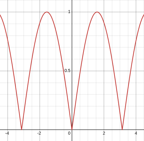
abs(sin(x)) appears to bounce like downwards acceleration (Desmos)

mix (lerp)

mix (often called lerp or “linear interpolation”[0]) lets you mix two things together. It works on two floats, vec2s, vec3s, etc. All you need to do is give it a number between 0.0 and 1.0 (inclusively) and it will mix the two things together.

Above, when t is 0.0, it will be red, when t is 1.0, it will be blue. If t is in the middle, then the color will be in the middle.

mix also can handle values outside of 0.0 and 1.0. I leave it as an exercise for the reader to figure out (or imagine yourself) what happens in that case.

Masking

Image- and video-editing software use masking to show one image/video over part of the screen and another image/video over another part of the screen. This effect is simple to replicate in graphics. The way it works is you first get some number to be 0.0 for the UV coordinates where you want one effect and 1.0 for the other UV coordinates. Then, mix the two effects together using the mask.

In the example above, I used the expression radius < dist && dist < radius + 0.1, which checks if radius is less than dist and (&&) dist is less than the radius plus a small value. If you've never seen this, this kind of expression is testing whether some conditions hold and gives you either true or false, which is something we call a boolean (bool). The use of the float(...) converts that true/false into a number, 1.0 for true and 0.0 for false.

That second to last line painting(uv) * one_minus(mask) + painting(-uv) * mask is also fairly common. Similar to the red/blue example with mix, we are adding the two colors together. However, we know that one of mask and one_minus(mask) will be 1.0 and one will be 0.0. So one of the colors will be vec3(0.0, 0.0, 0.0) (black) and one will be the actual color we want to display for that part of the screen. Adding black has no effect since it's represented by all zeros.

This interactive example above is not too dissimilar from the visualization we had in the introduction when I was explaining that the color for each part of the screen is decided independently. We break up the UV coordinates into chunks using floor, then choose a random value between 0.0 and 1.0 for each chunk. The mask is just using the rand < 0.5 condition to randomly select half of the chunks as 1.0 and half as 0.0. We know this will happen because asking random for a number gives us a number that's roughly 50% chance of being above 0.5 and 50% below. Adding mod(rand + time, 1.0) constantly shifts the mask, so which squares have a value above/below 0.5 changes.

It's almost like how they fade between scenes in Star Wars. In this interactive example, if you remove the changes to y_step, then mask is just comparing uv.x and uv.y:

float mask = float(uv.x < uv.y);

mask flips from 0.0 to 1.0 when uv.x becomes greater than uv.y or, when our UV coordinate is further to the right than it is above the bottom. So the lower part of the mask is when uv.x is bigger (mask is 0.0) and the upper part is when uv.y is bigger (mask is 1.0).

Now go look at the original again. The part where we use floor (or sin01 in the line that starts with //) simply applies some small changes to y_step before we do the comparison for mask.

This mask looks complex, but it's very similar to the interactive example above this one. The key to understanding it is we take uv.y, use mod to cycle between the numbers 0.0 and size (mod(threshold, size)), and then use mask to split it half-half (float(threshold < size / 2.0)) between the normal painting and a painting that's been pushed down (painting(uv + vec2(0.0, 0.01))). time makes the mask slowly move and sin01 adds the up-and-down detail to the mask.

min and max

min takes two numbers and gives back whichever is less. max takes two numbers and gives back whichever is more. It also works on vec2, vec3, etc (as seen above). In that case, min and max work on the individual .x, .y, and .z. So these two lines are equivalent:

color = min(p1, p2);
color = vec3(min(p1.x, p2.x), min(p1.y, p2.y), min(p1.z, p2.z));

min and max can act as a simple way to blend colors together, like blend modes in an image-editing program (see the interactive example above). The most common reason I use them is to ensure that I don't get back anything less than 0.0 or more than 1.0. For example, dividing a number by 0 is not something you should do. So, if you have an expression like a / b, and you think sometimes b could be 0.0, you could write a / max(0.001, b), so once b dips below 0.001, 0.001 will be the greater of the two numbers.

clamp

Using clamp is like using both min and max. In the interactive example above, when uv.x is more than 0.8, it will simply be 0.8. When it is less than 0.2, it will be 0.2.

The reason we have the stretched lines look in the interactive example above is because the clamp makes all the uv.x on the far left have the same value and all the uv.x on the far right side have the same value. uv.y is unaffected, so for those changed UV coordinates, we are essentially grabbing the same vertical line from painting over and over (either where uv.x is 0.2 or 0.8).

map (remap)

map (or remap in some contexts) takes a number from one range and changes it to the equivalent number in another range:

float map(float value, float min1, float max1, float min2, float max2) {
    return min2 + (value - min1) * (max2 - min2) / (max1 - min1);
}

What 😕? Let me explain. Suppose you have the range 0.0 to 1.0 and you have the number 0.5. That number is halfway between them. If your second range is 1.0 to 10.0, halfway between them is 5.5. So, map(0.5, 0.0, 1.0, 1.0, 10.0) is 5.5. If the number was 0.0, then map would give us 1.0, because 0.0 is at the beginning of our first range (0.0 to 1.0) and 1.0 is at the beginning of our second range.

In part 1, we defined something called sin01, which is like sin but the range is 0.0 to 1.0:

float sin01 (float value) {
    return (sin(value) + 1.0) * 0.5;
}

We could also use map to write sin01 instead, where the result of sin is mapped into the range 0.0 to 1.0:

float sin01 (float value) {
  return map(sin(value), -1.0, 1.0, 0.0, 1.0);
}

Exercise for the reader: How would you write map using mix?

sin01ma

Those hills are really rolling! sin01ma is an abbreviation for “sin, multiply, add”:

float sin01ma (float t, float period_secs, float offset_secs, float m, float a) {
    return sin01((t + offset_secs) / period_secs * 2.0 * PI) * m + a;
}

As I mentioned in part 1, changing a value from 0 to 1 is like turning something from off to on, or transitioning something completely from one way to another way.

sin01ma is like sin or sin01, but you tell it how often it should repeat (period_secs), how far into that cycle it should start (offset_secs), a number to multiply the sin01 by (m), and finally a number to start at (a). So sin01ma(time, 2.0, 1.0, 3.0, 4.0) will move back and forth between 4.0 and 7.0 (4.0 + 3.0) every 2.0 seconds, but start 1.0 second “fast-forwarded” into that cycle.

I came up with sin01ma based on an observation in my work that I often layer multiple effects in the videos, each one repeating on an interval and staggered so the layered effect wouldn't seem to repeat so quickly. Like several different pendulums swinging together. That's why sin01ma takes the period_secs... to express how often you want it to cycle between a and a + m. And the offset_secs helps you to stagger the effects so that they don't all stop and repeat at the same time (offset_secs should be between 0 and period_secs).

Here's an example layering effects. This time, there are two effects with different period_secs and offset_secs. The stretch on the .x dimension repeats every 2.05 seconds and the stetch on the .y dimension repeats every 3.0 seconds (but fast forwarded 0.1 seconds). Just these minor changes can produce a lot of unique behavior.

Now imagine if we used sin01ma to calculate m or a... with a large period_secs and small m, you can basically “wiggle” a value very slowly over a long period of time.

stay01

stay01 is like sin01, but it stays most of the time at 0 or 1, transitioning quickly between them. Like sin01ma, it also takes period_secs and offset_secs to make it easier to stagger them and repeat using different intervals.

I created stay01 because I wanted to try something besides sin (or mod) for cycling between 0 and 1 to turn on and off effects. In animation software, you can adjust the “ease” with which you transition the character's pose from one to another to make it more lifelike or cartoony. In video- and audio-editing software, you can adjust how fast a fade transitions to establish a different feeling. So why not in graphics effects?

float stay01 (float t, float period_secs, float offset_secs, float power) {
    float wave = sin((t + offset_secs) / period_secs * 2.0 * PI);
    float s = sign(wave);
    float a = map(s - (s * pow(1.0 - abs(wave), power)), -1.0, 1.0, 0.0, 1.0);
    return a;
}

stay01 is defined using the observation in math that anything between 0 and 1 that's not 1 will move towards 0 if you multiply it by itself. For example, when 0.5 is multipied by itself ten times, it's about 0.00098 😲. This has a flattening effect on things like sin, but since our objective is for it to “stay” or flatten around 0 and 1, we have to flip sin so the parts we want flattened are close to 0 when we flatten it, then reverse flip it again so the flattened parts are around the highest and lowest parts of the original sin, then map that value between 0 and 1 🫠 (don't worry if that's not intuitive... it took a bit of thinking to figure it out):

stay01 becomes flatter and the transition faster as you increase the power (Desmos)

Finally, the strength just tells stay01 the power to use when flattening (how many times to multiply by itself). With a strength of 1, it's just sin01. I typically use 3 to 5 to create a fast but smooth transition. Higher strength tends to make the transition too fast, but might be necessary if period_secs is large.

Warping UV coordinates

painting repeats itself

I apologize for not explaining this in part 1. You probably already have noticed that when UV coordinates have a .x or .y below 0.0 or above 1.0, painting just repeats on the other side. It's as if painting first does uv = mod(uv, 1.0) before looking up these UV locations on painting. This behavior can be changed, but it's outside the scope of this article.

This is also why occassionally I'll use something like uv = mod(uv, 1.0) because in a previous step, I multiplied the UV coordinates to create a grid pattern. If we don't use mod here, many of the UV coordinates will be above 1.0 and that may not work for the next effect.

The order that you change the UV coordinates matters

You'll often want to apply two effects, one after the other, to the UV coordinates. But you discover that it doesn't look right, until you reverse the order in which you apply them. An example is you want to apply some effect to the UVs and then duplicate it into a five by five grid. You start by applying the effect (e.g. uv + pow(uv.y, 5.0)) and then shrinking it down (mod(uv * 5.0, 1.0)) into multiple copies in a grid. But it doesn't look right:

If the effect is not what you expected, try reversing the order that you change the UVs:

pow

pow raises a number to another number (exponentiation). So pow(4.0, 2.0) will give you the same as 4.0 * 4.0. Raising a value to an exponent less than 1.0, even less than 0.0, is totally valid.

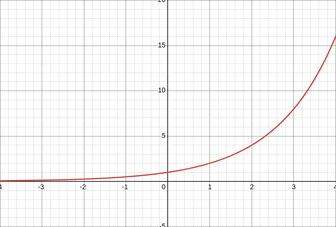
pow(2.0, x) for negative x never quite reaches 0.0 (Desmos)

As I noted with stay01, raising a number to an exponent brings decimals between 0.0 and 1.0 closer to 0.0. This is useful for creating bulges or very strong curves or compression or stretching. Used in conjunction with one_minus, you can flatten values against 1.0 by first subtracting the number from 1.0, using pow, then substracting that again from 1.0: one_minus(pow(one_minus(uv.x), 10.0))

In the above effect, the use of the two one_minuses seems to reduce the effect as uv.x approaches 1.0.

Exercise for the reader: Remove the outer one_minus. What happened? Why?

As you may have seen in the definition of stay01, you can use pow, sign, and abs together to multiply a number that might be negative by itself many times and keep the positive/negative sign: sign(value) * abs(pow(value, exponent)). No matter what value and exponent are, the result will always be positive if value is positive and negative if value is negative.

rotate

rotate will rotate vec2s around vec2(0.0, 0.0) (the origin). What that means is if your UV coordinate is at vec2(0.0, 0.5) (halfway up the left side), rotating it 90° degrees (about 1.5 radians) will give you vec(0.5, 0.0) (halfway along the bottom). It's like you stuck a pin in the lower left corner and used your finger to slide it around the pin.

vec2 rotate(vec2 v, float angle_radians) {
    float s = sin(angle_radians);
    float c = cos(angle_radians);
    mat2 m = mat2(vec2(c, s), vec2(-s, c));
    return m * v;
}

However, in the interactive example above, it's rotating around the center. THAT'S WEIRD. ULYSSE, DIDN'T YOU JUST SAY SOMETHING ABOUT ROTATING AROUND THE BOTTOM LEFT CORNER?? Correct. If you want to rotate painting around the center, you have to first change all the UV coordinates so that the center is at vec2(0.0, 0.0). Just subtract vec2(0.5, 0.5), rotate your UV coordinates, and then add the vec(0.5, 0.5) back in.

circle_sdf and rect_sdf

SDF stands for signed distance field, which in this context is a fancy way to say distance from the edges of a shape. Suppose you want to know how far each UV location is from the edge of a circle. One way to do that is to first figure out how far your UV location is from the center of the circle. For example, if the center of your imaginary circle is at vec2(0.5, 0.5) and your UV is vec2(0.6, 0.5), then the distance is 0.1. Then, subtract the radius of the circle. So if the radius is 0.3 and your UV is 0.1 from the circle's center, that gives you -0.2. Huh. Therefore, this UV is -0.2 from the edge of the circle (negative values are inside the circle). This is how circle_sdf works:

float circle_sdf (vec2 uv, vec2 center, float size) {
    return distance(uv, center) - size;
}

Others have figured out clever ways to quickly calculate the signed distance fields for many basic shapes. Inigo Quilez's list is the best I've seen. Another common one is the rectangle (which I won't explain because Inigo Quilez has a great video on it):

float rect_sdf (vec2 uv, vec2 center, vec2 size) {
    vec2 d = abs(uv - center) - size;
    float outside = length(max(d, 0.0));
    float inside = min(max(d.x, d.y), 0.0);
    return outside + inside;
}

rect_sdf will give you the distance from your UV to the closest edge of the rectangle. In general, parts of the SDF that are close together will have distances that are similar, making these great for warping UVs, or even color:

There are also ways to blend between multiple shape SDFs. One way is to use the average of the distances. If we averaged the distance a UV is from an imaginary circle and the distance that same UV is from an imaginary retangle, we might get some shape that's in-between.

Another approach is to take the min of the distances, which is effectively a union of the shapes. Last, there's smin (smooth-min), which I copied from Inigo Quilez.

float smin (float a, float b, float k) {
    float res = exp2(-k * a) + exp2(-k * b);
    return -log2(res) / k;
}

smin also unions shapes together, but also seems to create some kind of webbing between them, looking a bit more organic. The k that smin accepts is like a tightness factor... higher values (10.0+) seem to pull pull everything closer together, whereas lower values (2.0, 3.0) spread out and combine more. smin is what I used to combine 3D shapes together in my interactive video essay, Acceptance.

Try out different ways of combining circle_sdf and rect_sdf or even two circle_sdf or two rect_sdf together.

xy_to_r_theta and r_theta_to_xy

It's not exactly a kaleidoscope, but it's still quite mesmerizing! So far, the UV coordinates have always had .x representing how far to the right and .y representing how far up (the cartesian coordinate system). An alternative coordinate system, polar coordinates, describes positions as distance from the center (r) and rotation around the center (theta θ).

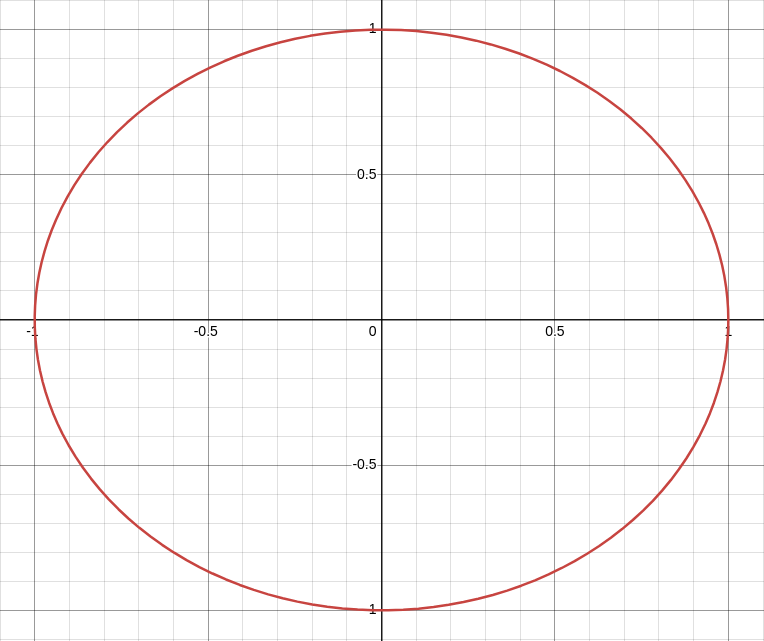
The line drawn when the r = 1 and θ can take on any value in polar coordinates (Desmos)

Much like the rgb2hsv ↔ hsv2rgb combination, you can convert between cartesian and polar coordinates using xy_to_r_theta and r_theta_to_xy.

vec2 xy_to_r_theta(vec2 xy) {
    float r = length(xy);
    float theta = atan(xy.y, xy.x);
    return vec2(r, theta);
}

vec2 r_theta_to_xy(vec2 rt) {
    float r = rt.x;
    float theta = rt.y;
    return vec2(r * cos(theta), r * sin(theta));
}

They can be used as an alternative to rotate by first converting to polar, changing θ, and then converting back to cartesian. But remember that polar coordinates measure the distance and rotation using the center, which is not vec2(0.5, 0.5), but vec2(0.0, 0.0). Therefore, like rotate, if we want to rotate something around the center of painting, we must first subtract vec2(0.5, 0.5) before converting to polar coordinates and then add vec2(0.5, 0.5) after converting from polar coordinates.

The most interesting line in the interactive example above is theta = mod(theta, slice), the polar coordinates equivalent of using mod to repeat the same UV square everywhere. Each slice of the polar coordinates pretends that it's the first slice using mod, so every slice looks the same after we convert back.

Textures can warp UVs

In the introduction, we talked about what textures are. painting is a texture... an image that's loaded onto a 3D model. And textures like painting have a lot of distinct, natural shapes that we might recognize. This can make for a great way to modify UV coordinates, especially using the colors for a texture image to warp the UV coordinates for that same texture! It's like some kind of stencil or green screen trick.

Changing things together looks consistent

Something I discovered was that many things blend well together if you identify which aspects are most contrasting and make them the same. In this interactive example, it's easy to identify that there's something rotating because the borders of painting are quite clear. But it's much harder to tell that there are two paintings overlapping because they are moving together and the colors are averaged together in greyscale. If we just used mix like this:

color = mix(
    painting(rotated_uv1),
    painting(rotated_uv2),
    0.5
);

then the green of the hills mixing with the blue of the sky gets a bit muddled. Try replacing the last four lines of the interactive example above with this mix expression. Using the averaged color, it seems as if there was ever only one painting.

Noise

Noise is hugely impactful in 2D/3D animation and game development for imitating and adding detail, as well as creating new forms out of nothing. Noise usually expects you to give it a UV coordinate and it gives back a number between 0.0 and 1.0 (but never exactly 1.0, except for voronoi_noise). You can zoom in or zoom out on noise by multiplying your UV coordinates by a number before creating the noise.

In the interactive example above, we see four different kinds of noise and then we mask them so each only shows up in one part of the screen. In the past, our masking only separated two things on screen, but there's no reason why you can't mask as many things as you want if you can make a check for each mask.

Since noise is always between 0.0 and 1.0 and UV coordinates near each other usually produce noise values that are close together, noise can be used in any of the same places as the techniques in Working with 0 and 1 or Warping UV coordinates.

Some of the noise functions are quite long, so I haven't included them here, but you can find them here.

In the example above, I've set the noise to turn on and off with stay01 so you can see how adding different noise to the UV coordinates affects painting.

white_noise

We've actually already used white_noise with random, which is just a form of white_noise. white_noise is like TV static, where you shouldn't expect to see any patterns.

As defined for our usage, white_noise is actually a bit more general. white_noise takes in float, vec2, or vec3 and gives back the same type of thing that you gave it. So white_noise(vec3(0.0, 1.0, 2.0)) will give a vec3. Therefore, random is usually best to use with UV coordinates.

white_noise is not without its uses, as we've seen with random. If you reduce the effect of random by multiplying it by a small number, it can create a sanded, blurring, jitter effect.

simple_noise, perlin_noise, turbulence_noise

The other kinds of noise all have more recognizable patterns. Above is the first example from the Masking section with simple_noise added. Since simple_noise has a recognizable clumpy/smoky pattern, it comes through visually when calculating the distance between uv and the center, almost like water spilling over a bumpy table.

Depending on the situation, you'll often want to map the noise so that it can be negative as well. If you're only adding positive numbers to UVs, it tends to push everything in one direction, creating more asymmetry.

perlin_noise has more distinct structure compared with simple_noise and is good for many things including smoke and glass. The perlin_noise gives painting a real painted look 😅.

perlin_noise can give imagery a glassy look as well. Here, we've applied white_noise (random) to create a rough, scratchy look on a finer detailed level and perlin_noise to add somewhat of a paint-strokes/glassy look. We added the white_noise to the UVs that we used to generate the perlin_noise. We didn't have to do this; we could have added them to the UV coordinates separately, but this way looked better, so I kept it.

turbulence_noise is what happens when you apply perlin_noise several times, each time making lighter changes and at a finer detail. turbulence_noise is great for things like fire, smoke, dissolving, and fluids. It takes the UV coordinate and a number that represents how many times to layer perlin_noise. You probably don't need that number to be that high. I have been using 5.0.

In the example above, t slides back and forth between 0.0 and 1.0 and we use a small band of that (t to t + 0.1) to display a mix of yellow and orange.

A water look can be made by combining multiple noise values together. It's fascinating because at a glance, your eyes think it's water, but once you follow the movement with your eyes, it's easy to pick out some noise moving down and other noise moving left.

voronoi_noise

Imagine you randomly toss a handful of seeds onto the ground. You take a photo looking down at them and then darken the parts of the photo based on how far they are from the nearest seed. That is what voronoi_noise (worley noise) approximates. There are dark spots where those theoretical seeds are (distance 0.0 from the nearest seed) and then the color gets whiter as you get further from the nearest seed.

When you one_minus voronoi_noise, you get rounded-looking surfaces. voronoi_noise is wonderful at scattering and partitioning things, whether it's biological cells, eyeballs, marble, camouflage, cracked materials, or stars.

By applying pow to voronoi_noise once you've one_minused it, most of the parts that are far from any seeds/focal points will flatten to 0.0 and what's left are the parts that are very close to 1.0, the areas around the seeds.

In the example above, I've also added some flicker to the stars by rolling some simple_noise across it that will decrease the brightenss. Because the values from simple_noise transitions slowly between 0.0 and 1.0, the flickering won't be too jarring. Also since stars are far apart, the large patterns in the simple_noise flowing by are barely noticeable.

Changing the color

replace_rgb

In my research on how game developers create stylized aesthetics, a common technique is to drastically limit the color palette and/or bring out certain colors in parts of characters/objects where they don't normally show up as much. Borrowing from this idea, replace_rgb simply takes a color and replaces each of its red, green, and blue with new colors:

vec3 replace_rgb (vec3 old_color, vec3 new_red, vec3 new_green, vec3 new_blue) {
    return new_red * old_color.x + new_green * old_color.y + new_blue * old_color.z;
}

The .x of old_color determines how much new_red there will be, .y how much new_green, and .z how much new_blue. If you look at the colors I chose in the example above, you'll notice that each vertical column of numbers add up to 1.0:

vec3 new_red   = vec3(0.0, 0.5, 0.5);
vec3 new_green = vec3(0.5, 0.0, 0.5);
vec3 new_blue  = vec3(0.5, 0.5, 0.0);

This is not a requirement, but ensures that replace_rgb will never give you a color with any of red, green, or blue higher than 1.0. Consider what would happen if the new colors you gave replace_rgb were all white:

vec3 new_red   = vec3(1.0, 1.0, 1.0);
vec3 new_green = vec3(1.0, 1.0, 1.0);
vec3 new_blue  = vec3(1.0, 1.0, 1.0);

A grey color (vec3(0.5, 0.5, 0.5)) passed to replace_rgb with these white replacement colors would end up as vec3(1.5, 1.5, 1.5). Going over 1.0 means you'll lose detail in the image. That might be what you want... to distort the lighter colors.

rainbow_gradient

rainbow_gradient's usage was covered in part 1.

const vec3 rainbow_colors[7] = vec3[7](
    vec3(1.0, 0.0, 0.0),
    vec3(1.0, 0.5, 0.0),
    vec3(1.0, 1.0, 0.0),
    vec3(0.0, 1.0, 0.0),
    vec3(0.0, 0.0, 1.0),
    vec3(0.29, 0.0, 0.51),
    vec3(0.93, 0.51, 0.93)
);

vec3 rainbow_gradient (float value) {
    value = clamp(value, 0.0, 1.0);
    float segment = 1.0 / 6.0;
    float segment_index = floor(value / segment);
    float segment_value = fract(value / segment);
    vec3 color1 = rainbow_colors[int(segment_index)];
    vec3 color2 = rainbow_colors[int(segment_index + 1.0)];
    return mix(color1, color2, segment_value);
}

rainbow_gradient essentially places the ROYGBIV colors on the range 0.0 to 1.0. Next, it finds the two closest colors to value in that range and mixes them together according to value.

rgb2hsv and hsv2rgb

rgb2hsv and hsv2rgb's usage were covered in the end of part 1. Don't underestimate the power of desaturating a bit and changing the hue. It can push things towards the Uncanny Valley.

Above, min and max keep the saturation from getting too low max(0.0, hsv.y - 0.2) or the brightness too high min(1.0, hsv.z + delta), while mod (as shown in part 1) takes advantage of the fact that a color with hue of 0.0 is the same as with 1.0, so wrapping around from 1.0 back to 0.0 with mod doesn't create a jarring look.

vec3 rgb2hsv(vec3 c) {
    vec4 K = vec4(0.0, -1.0 / 3.0, 2.0 / 3.0, -1.0);
    vec4 p = mix(vec4(c.bg, K.wz), vec4(c.gb, K.xy), step(c.b, c.g));
    vec4 q = mix(vec4(p.xyw, c.r), vec4(c.r, p.yzx), step(p.x, c.r));

    float d = q.x - min(q.w, q.y);
    float e = 1.0e-10;
    return vec3(abs(q.z + (q.w - q.y) / (6.0 * d + e)), d / (q.x + e), q.x);
}

vec3 hsv2rgb(vec3 c) {
    vec4 K = vec4(1.0, 2.0 / 3.0, 1.0 / 3.0, 3.0);
    vec3 p = abs(fract(c.xxx + K.xyz) * 6.0 - K.www);
    return c.z * mix(K.xxx, clamp(p - K.xxx, 0.0, 1.0), c.y);
}

Credit for these goes to Sam Hocevar's post.

palette

palette takes a number t between 0.0 to 1.0 and some colors to get a color along some continuous color gradient/spectrum. It's a good alternative to rainbow_gradient. Credit goes to Inigo Quilez, who has an explanation on it.

vec3 palette (vec3 a, vec3 b, vec3 c, vec3 d, float t) {
    return a + b * cos(6.28318 * (c * t + d));
}

Averaging colors to create new colors

A lot of my thinking in this medium focuses on keeping the features in the final image transitioning smoothly, so it doesn't look like sharp, granular noise. The techniques in Warping UV coordinates can do that very well.

But it's not the only way. In the interactive example above, I use chromatic aberration to shift red, green, and blue versions of painting apart (as we've seen before), but then instead of simply putting .x, .y, or .z in a new color, I average the three color amounts together. This still maintains a relatively slow-transitioning image if the amount you shift the red, green, and blue apart is small. Like colors will still be relatively close together.

But averaging them together is like a blur. It produces a single, mixed value. And what can we do with a number between 0 and 1? Use it with rainbow_gradient or palette, or even feed it into any other place where that number turns on/off an effect (Working with 0 and 1). For example, mix two colors together using the average we just calculated to determine how much of one color and how much of another.

You can hear more from me on YouTube or Twitter.

Footnotes

[0] The “linear” in “linear interpolation” implies that when mixing values together, it linearly transitions between them along a straight line (as opposed to something like sin or y = x * x which will be curved.